matHUMANtics Algebra

linear transformation image and kernel

Linear Algebra

These are my notes from working through various texts and handbooks of linear algebra. The main source is linked below.

Linear Algebra Handbook

************************************************************************

FAQ or "Who invented linear equations? We should go back in time and kill them!"

  1. Who uses lines or linear equations?
  2. What is linear algebra?
  3. What are lines good for?
  4. What are some examples of phenomena that can be modeled by linear equations?
  5. What makes an equation linear?
  6. When will I ever use linear equations?
  7. When were linear equations invented?
  8. Why does a linear equation produce points that fall on a straight line?
  9. Why do some sets of points fall on a straight line?
  10. Why do we use the term linear for some equations?
  11. Why are linear equations important?
  12. How can we recognize when a pattern is linear?
  13. How do we solve linear equations?
How does my mom know how much gas to put in the car when we stop at the filling station?
Your mom's car has a tank inside of it which holds the gas needed to drive it. She knows the volume of the gas tank in her car. Do you? To begin, let's say the volume of the gas tank is 14.5 gallons. When she goes to fill up the tank with gas, your mom knows to stop the gas pump before the meter reads 14.5 gallons.
What happens if she forgets to stop pumping before the meter reaches the 14.5 gallon mark?
Today, most filling stations have pumps that automatically stop before the tank volume is exceeded. If that fails, then the tank will overflow, causing gas to spill on the ground and be wasted.

How much gas can she buy with 20 dollars? Why doesn't she buy that much?

How many times will we have to fill the car on our road trip from California to Colorado?

Why do the points (gallons of gas, cost) always seem to fall on a line?

Why does every equation describing a gas cost vs. volume relationship make a line?

Why does every equation of the form y = mx have a line for its graph?

What is the relationship between a person's height and their shoe size?

How can linear equations help me make good decisions? Suppose you want to know how many hours you will have to work to earn a certain amount of money. Suppose you want to know what quantity of an item you can afford. Suppose you want to know the break even point between two internet services so you can decide which is the best value short term vs. long term. Suppose you want to predict annual migration between different cities. Suppose you want to determine a polynomial model to fit a data set. Suppose you want to balance a chemical reaction.


Why Linear Equations? ************************************************************************-->

Linear Systems from Antiquity

Now that you have studied the properties of linear functions you are ready to begin the study of systems of linear equations. A clay tablet found in Iraq, dating around 300 BC, poses the following problem.

There are two fields whose total area is 1800 square yards. One produces grain at the rate of ⅔ of a bushel per square yard while the other produces grain at the rate of ½ a bushel per square yard. If the total yield is 1100 bushels, what is the size of each field?
MacTutor

There are two unknowns in this problem: the area of each field. Let x = the area of the first field and let y = the area of the second field. Two equations are required to describe the situation: x + y = 1800 and (⅔)x + (½)y = 1100. Multiplying both sides of the second equation by 6 gives us the equivalent equation 4x + 3y = 6600. Each equation describes a line. The solution of this system is the point whose coordinates solve both equations simultaneously, that is, this point is the intersection of the two lines described. A linear system can be solved by various methods: interpolation, graphing, substitution, elimination, or matrix methods.

Looking at the system again, we see that there are six numbers to deal with. Arranging them into a rectangular array looks like the following.

LaTeX

Interpolation:

Guess 1: If x = 900 and y = 900, then x + y = 1800 and 4x + 3y = 6300.
Guess 2: If x = 0 and y = 1800, then x + y = 1800 and 4x + 3y = 5400.
Guess 3: If x = 1800 and y = 0, then x + y = 1800 and 4x + 3y = 7200.
Guess 4: If x = 1400 and y = 400, then x + y = 1800 and 4x + 3y = 6800.
Guess 5: If x = 1100 and y = 700, then x + y = 1800 and 4x + 3y = 6500.
Guess 6: If x = 1200 and y = 600, then x + y = 1800 and 4x + 3y = 6600.

Graphing:

Substitution: Solving the first equation for y gives us y = 1800 − x. We then substitute 1800 − x for y in the second equation to get 4x + 3(1800 − x) = 6300. This tells us that x = 1200. By substituting 1200 for x in the first equation, we see that y = 600.

Elimination: If we multiply the first equation by −3, then we get the equivalent system −3x − 3y = −5400 and 4x + 3y = 6600. By "adding" the equations, we get x = 1200. So, y = 600.

Matrix Methods: The rest of the linear algebra portion of this book will introduce and explore these in more detail than you thought possible or want.


The Method of Determinants

To begin our treatment of determinant methods for solving linear systems, we would like to consult the classic text, Ars Magna, published in 1845 by scoundrelous physician and intentional curmudgeon, Girolamo Cardano.

Cardano poses the following problem.

Three men had some money. The first man with half the others' would have had $32; the second with one-third the others', $28; and the third with one-fourth the others', $31. How much had each?

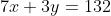
From this, we get the 3 × 3 linear system

LaTeX
LaTeX
LaTeX

No, Charly, the language is not weird, its English. Yes, Charly, that's not even a lot of money for one man, nevermind three. That's not the point. Where were we? Let's get back to it, shall we? After solving the third equation for z, Cardano reduces the problem to solving the 2 × 2 linear system

LaTeX
LaTeX

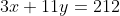
He then chooses to use the tried and true rule for four proportional quantities on the second equation to obtain the equivalent system

LaTeX
LaTeX

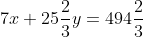
We can see what he's going to do next. He suggests this means

LaTeX

which gives us

LaTeX

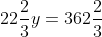
Thus, the second man's share of the money is y = $16. Using this result on the original first and second equations, he gives us the second 2 × 2 system

LaTeX
LaTeX

Illustrating the same technique as before, Cardano tells us that the third man's share is 24. After solving the original first equation with the knowledge that the second and third men have $16 and $24, respectively, he determines that the first man has $12. He then concludes with a suggestion for general practice, "One term must always be reduced to have the same coefficient, and then the difference between the numbers is necessarily the difference between the other term...." Today, this method of solving systems is called elimination. It leads us quite naturally to the notion of determinants. But first... Cramer!

In contrast to Cardano, Gabriel Cramer was an affable scholar. He is credited with the now infamous Cramer's Rule taught to lucky high school math students. However, the treatment given of his rule in high schools is appallingly distilled. We will look at his book Introduction A L'Analyse Des Lignes Courbes Algébrique to get the real story which follows Cardano's work. A partial translation into English can be found here.

*********************************************************

Consider the general 2 × 2 linear system

LaTeX

The method of elimination gives us the solution

LaTeX

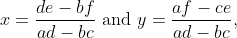
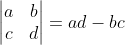
provided ad − bc is nonzero. Why is it necessary to say the denominator can't be zero? The numerators and denominator of the solution are commonly interpreted as something called a determinant. For a 2 × 2 matrix

LaTeX

the determinant of A is denoted by det(A) or |A| and is given by

LaTeX

Now, let's look at the system of equations as the stack of equations

LaTeX LaTeX

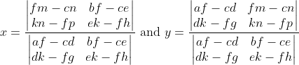
Notice that the numerators and denominators of the solution look like determinants of matrices. That is, we may write

LaTeX

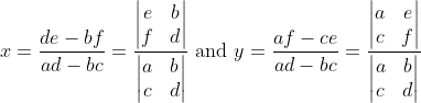
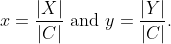
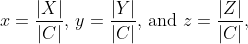
We see that the denominator of x and y is the determinant of a matrix C of the coefficients of the linear system. Furthermore, the numerator of x is the determinant of a matrix X we get by replacing the column of coefficients of x in C by the column of constants, and we define a matrix Y analogously. More precisely, let

LaTeX

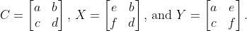
Thus, we may write the solution more elegantly as

LaTeX

This formulation of the solution of a linear system into ratios of determinants is called Cramer's Rule. Its elegance allows us to solve 2 × 2 linear systems by mental calculation. Let's apply it to three different systems to see what else we may learn.

Example 1: Solve the system

LaTeX

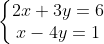
Solution: Three quick mental calculations tell us that

LaTeX

Example 2: Solve the system

LaTeX

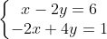
Solution: Immediately, we run into the problem of division by zero, for |C| = 0 and thus x and y are undefined. What does this mean about the system? A quick inspection of the slopes and intercepts of the lines described reveals why this system has no solution.

Example 3: Solve the system

LaTeX

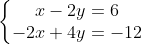
Solution: We run into the same problem of |C| = 0, but the slopes and intercepts of this system lead us to conclude that it has infinitely many solutions.

Naturally, we have some questions.

  1. Is the determinant of the coefficient matrix of a linear system being nonzero sufficient condition for the system to have a unique solution?
  2. Is it a necessary condition?
  3. What are the necessary and sufficient conditions for a linear system to have infinitely many solutions or have no solution?
  4. What do we mean by sufficient condition and necessary condition?

After enough practice using Cramer's Rule for 2 × 2 linear systems, we begin to notice that we can completely characterize their geometry in terms of the determinants of their matrices. How much practice is enough? That depends on who's asking. A 2 × 2 linear system describes

  1. two lines intersecting at a unique point if and only if |C| ≠ 0
  2. two parallel lines if and only if |C| = 0 and |X| ≠ 0, and
  3. one line if and only if |C| = 0 and |X| = 0.

If you don't understand this, it's because you haven't yet practiced enough. Keep at it and you will understand. But first, a word of caution... algebra hides the geometry of whatever it concerns itself with because it is designed to encode spatial relations. Thus, we must always bother to visualize the geometry being described by algebraic statements.

Another question arises. Can Cramer's Rule be generalized to solve n × n linear systems? Let's explore the solution of the general 3 × 3 linear system

LaTeX

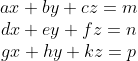
By eliminating z, we get the following reduction to the 2 × 2 linear system

LaTeX

The solution is given by Cramer's Rule:

LaTeX

The determinants give us

LaTeX

After distributing, alphabetizing factors, combining like terms, and cancelling the common factor, we get

LaTeX

What a mess! Wouldn't it be beautiful if that mess turned out to be

LaTeX

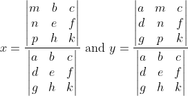
much like it is in the 2 × 2 case? To proceed, we will first have to return our attention to the definition of determinant because it's not yet clear how we may compute these 3 × 3 determinants. I will leave it to you to understand why we define determinants as we do since it usually proves to be a rather tedious exercise in solving linear systems. We could just proceed from the belief that whatever a determinant is, it is certainly based on the denominators of solutions of linear systems, a fact which led us to interpret the numerators as determinants as well. There also seems to be a recursive quality to solving the 3 × 3 system -- we reduced it to a 2 × 2 system -- so we may as well look for a similar recursion in exploring the determinant of a 3 × 3 matrix. Let's begin by noticing that some pairs of terms in the denominator of x have a common factor. Let's pretend for the moment that

LaTeX

In terms of 2 × 2 determinants, we may write

LaTeX
LaTeX
LaTeX
LaTeX
LaTeX
LaTeX

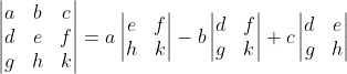
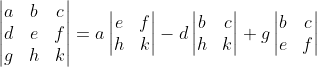
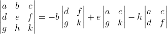
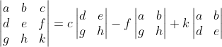
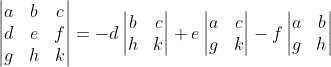
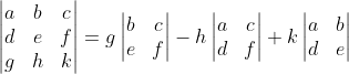
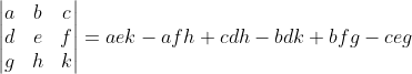
As it happens, there are only 6 distinct formulations of a 3 × 3 determinant into 2 × 2 matrices. Is there a counting formula for that? We shall see, but I digress. Back to the topic. Notice that each of these feature the entries in a single row or column, and each entry is multiplied by the determinant of the 2 × 2 matrix we get when the row and column containing that entry is excluded. For example, the entries of the determinant multiplied by a is found by removing the entries a, b, c found in the row of a and the entries d, g found in the column of a. That leaves the matrix

LaTeX

We call its determinant the minor of a, and we call a its cofactor. Through that lens, it is easy to see that each product in these 6 proposed formulations of the determinant of the coefficient matrix for the general 3 × 3 linear system contains a minor and its cofactor. Before we generalize this idea, we should take care to verify that a 2 × 2 determinant can also be characterized in this way. Have you convinced yourself? Great. Let's move on.

Question: What is the number of distinct expansions of an n × n determinant into (n − 1) × (n − 1) minors?

Recall that this exploration was dubious -- we pretended that 3 × 3 determinant was equivalent to the denominator of x. However, if we define the determinant of an n × n matrix to be precisely the denominator of the solution of the n × n linear system for which that matrix is the coefficient matrix, then we have defined a function on n × n matrices which seem recursively calculable as expansions into determinants of lesser dimension. We have determined this in the cases of 3 × 3 and 2 × 2 linear systems. There is, after all, nothing preventing us from doing just that. Why not run with it? We have this thing which comes out of the process of solving a linear system, and it turns out to be equivalent to a linear function of smaller such things we get from eliminating one variable from the original system. Yes, I am repeating myself because determinants are the intellectual equivalent of a briar patch: you can't get out without collecting more thorns.

Question: What effect does multiplication by a 2 × 2 matrix have on 2 and can we classify those effects in terms of determinants?

Problem: Prove that the system

LaTeX

has solution

LaTeX

where

LaTeX

whenever |C| ≠ 0.

Let's try this on a famous example. By 100 BCE, the Chinese had posed and solved the following problem.

There are three types of corn, of which three bundles of the first, two of the second, and one of the third make 39 measures. Two of the first, three of the second and one of the third make 34 measures. And one of the first, two of the second and three of the third make 26 measures. How many measures of corn are contained by one bundle of each type? MacTutor

There are three unknowns in this problem: the number of measures in one bundle of each type of corn.
Let x = the number of measures in one bundle of the first type.
Let y = the number of measures in one bundle of the second type.
Let z = the number of measures in one bundle of the third type.

This gives us the 3 × 3 linear system

LaTeX

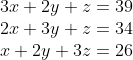
The Chinese solved this system using elimination on what they called a counting board. Thanks to European colonialism, that is now known as Gaussian Elimination on an augmented matrix. No, don't blame Gauss. Hate the game, not the player. Instead, we shall see whether the proposed extension of Cramer's Rule to the 3 × 3 case is useful. After setting up

LaTeX

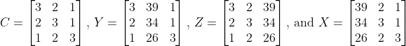
we see that |C| = 12 which tells us the system has a solution. Having a reason to proceed, we calculate |X| = 111, |Y| = 51, and |Z| = 33. So Cramer's Rule gives us

LaTeX

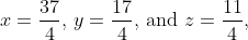
Questions: Were you able to obtain those fractions? Do they solve the system? If so, what does that tell us about determinants and Cramer's Rule? What is the geometry of 3 × 3 linear systems?

This determinant thing seems to be proving useful. Using elimination on a 2 × 2 system produces something we call a 2 × 2 determinant. Surprisingly, using elimination on a 3 × 3 linear system produces series of 2 × 2 determinants. Could it be that solving a 4 × 4 linear system will reveal a series of 3 × 3 determinants? I know I would rather not mess around with the general 4 × 4 case. The 3 × 3 case was messy enough. How about you? Perhaps there is a less tedious approach to exploring the generalization of determinants and Cramer's Rule.

We have already shown that the solution of a 3 × 3 linear system is computable in terms of 2 × 2 determinants that are evident from eliminating a variable to reduce the system to 2 linear equations in two unknowns. If we can somehow show that implies solutions of every system of higher order behave analogously, then we are in business. We will use a technique called mathematical induction which says that if a thing happens once, and that if it happening at all implies it will happen one more time, then it will happen every time. Well, that's the non-technical way of putting it. We shall be frighteningly technical from here on out. Suppose that

LaTeX

has solution

LaTeX

for |A| ≠ 0 and for each i from 1 to k, where A is the k × k coefficient matrix and Ai is the k × k matrix we get when the ith column of A is replaced with the column of constants d1 to dk. In other words, suppose that there is an integer k such that any k × k linear system has such solutions. Now, consider the system

LaTeX

Since we may reduce any (k + 1) × (k + 1) linear system to a k × k linear system by eliminating any one of its variables, say xk + 1, then there are coefficients cij and constants hi such that

LaTeX

is the reduction of our (k + 1) × (k + 1) linear system. By assumption, this reduced system has solution

LaTeX

for |C| ≠ 0 and for each i from 1 to k, where C is the k × k coefficient matrix and Ci is the k × k matrix we get when the ith column of C is replaced with the column of constants h1 to hk. Substituting into the first equation of the (k + 1) × (k + 1) linear system gives us

LaTeX

which we may write as

LaTeX

It remains to show that

LaTeX

where B is the (k + 1) × (k + 1) coefficient matrix of the (k + 1) × (k + 1) linear system and Bk + 1 is the (k + 1) × (k + 1) matrix we get when the (k + 1)th column of B is replaced with the column of constants f1 to fk + 1.

To finish this proof, we need a working definition of determinants for square matrices of any size. Looking back, we see that the determinant of an n × n matrix M is given by

LaTeX

for a fixed integer i with 1 ≤ i ≤ n, where Mij is the ij entry of M and mij is its minor. We will show that this thing we are calling the determinant of an n × n matrix defines a unique function δ from ℝn × n to ℝ that satisfies

  1. δ(I) = 1.
  2. δ is linear in the rows of a matrix. In other words, if A, B, and D are n × n matrices, and Ai = cBi + c'Di, then δ(A) = cδ(Bi) + c'δ(Di).
  3. δ(A) = 0 whenever two adjacent rows of A are equal. [2]

I suppose I should hide this until I look up the proof, but where's the fun in that? I'll just leave it dangling loose. Maybe you'll figure it out before I do.


The Method of Gaussian Elimination on Augmented Matrices

Going back to the method of elimination, we see that we can safely do certain things to a system without altering its solutions. Given an m × n system of equations, we may interchange any two equations, scale an equation, or add an equation to the scalar multiple of another. Notice that each of those manipulations of a system of equations acts only to change the numbers in a row of its coefficient matrix augmented by the corresponding constant. Suppose A is the coefficient matrix and b is the column of constants. Then we call the matrix [A b] the augmented matrix of the system and we refer to the aforementioned actions on equations in the system as elementary row operations. It should be clear that the "counting board" used in Nine Chapters on the Mathematical Art is the augmented matrix of a 3 × 3 linear system, that elimination was performed by column operations analogous to the row operations we mentioned, and that substitution was used once the value of one variable was made explicit. However, if the contributors to Nine Chapters were to continue with column operations, the following augmented matrix would have been the result.

LaTeX

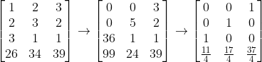
Today, we do practically the same thing, instead writing their first column as our first row, their second column as our second row, and their third column as our third row. Using row operations, we get

LaTeX

When considering why ancient Chinese mathematicians used column operations and solved for z first, we must keep in mind that they read and wrote in columns from top to bottom, then shifted left with each new column. However, we currently prefer to perform the row operations to solve for the leftmost variable. If, starting with the first row, we instead solved for x, then y, then z, we would see

LaTeX

In looking at the relative positions of the entries in the "counting board" and those in the augmented matrix, we are naturally led to the notion of the transpose of a matrix. For a matrix A, we denote its transpose by AT and define

LaTeX

After a bit of investigation, it becomes clear that the Chinese mathematicians back in 100 BCE were merely operating on the transpose of the matrix we would use to solve the same problem. Thus, it seems that performing row operations on a linear system S with augmented matrix [A b] gives the same solutions as performing column operations on [A b]T. We may wonder what other properties of matrices are not affected by the transpose. For example, we may want to compare |A| and |AT| for all square matrices. Yes, we should. No, don't try. There is no try. Only do.

Oh, yeah, we almost forgot... Gaussian Elimination. There's not much to say really. No offense to the memory of Karl Friedrich Gauss -- he was one of the greatest mathematicians in history --, but all he did in this story was put his Enlightenment stamp of approval on what the Chinese did 2000 years before him.


The Method of Elementary Matrix Products

It was Gauss who introduced the idea of matrix multiplication. Before we explore its applications to solving systems, we would like to know what insight led him to it. Let's reconsider what happens when we tranform a linear system by row operations.

Let's reconsider the problem of the corn bundles by asking whether a row operation can be the result of a matrix E acting on the augmented matrix [A b] of a linear system S. Gauss was most likely the first to explore this vein. What would that action be? Addition doesn't make sense, does it? Neither does subtraction for the same reason. Suppose there is a matrix M that acts on the augmented matrix of the corn bundle problem to perform the row operation of replacing row 2 with -2(row 1) + row 2. That is,

LaTeX

What size should M be? The most natural guess would be to make M the same size as the matrix on which it acts. Suppose

LaTeX

by some sort of multiplication. How could we define it? Let's try a straightforward multiplication, like

LaTeX

That gives us

LaTeX

Does that have any import? I don't think so either. Let's look at it this way.

LaTeX

Looking at it another way, we see

LaTeX

which gives us

LaTeX

if we pretend this matrix multiplication (whatever it is) distributes over matrix addition and that I is the multiplicative unit matrix (whatever THAT is). No harm in playing Dr. Frankenstein with boxes of numbers, eh?

LaTeX

Let's leave the growing monstrosity for a moment and ask a related and much simpler question. What is the multiplicative unit for


Vectors, Matrices and Systems of Linear Equations


Linear Independence, Span, and Bases


Linear Transformations


Determinants and Eigenvalues


Inner Product Spaces, Orthogonal Projection, Least Squares and Singular Value Decomposition


Special Matrices


Advanced Linear Algebra


Special Topics


Non-Linear Algebra

The Binomial Theorem

History

  1. (a + b)2 computed. Euclid. Greece. 4th century BCE. The Ongoing Binomial Revolution, David Goss, arXiv, 1105.3513v1, 18 May 2011

  2. LaTeX
    LaTeX
  3. First known presentation of binomial coefficients in a triangle. Pingala. India. 3rd century BCE. The Ongoing Binomial Revolution, David Goss, arXiv, 1105.3513v1, 18 May 2011
  4. Further triangular arrangement of binomial coefficients into a triangle. Halayudha. India. 10th century CE. The Ongoing Binomial Revolution
  5. Some more.... Al-Karaji. Persia. 953-1029 CE. History of Pascal's Triangle
  6. Known binomial theorem used to recreate Al-Karaji's triangle. Referred to as Khayyam's Triangle in Iran. Omar Khayyam. Persia. 11th century CE. History of Pascal's Triangle
  7. Triangular representation of binomial coefficients. Jia Xian. China. 11th century CE. History of Pascal's Triangle
  8. Yanghui's Triangle. Yang Hui. China. 13th century CE. History of Pascal's Triangle and The Ongoing Binomial Revolution
  9. A triangle of binomial coefficients was presented in a text of business calculations. Petrus Apianus. Europe. 1527 CE. History of Pascal's Triangle
  10. Tartaglia's Triangle. Niccolo Fontana Tartaglia. Italy. 1556 CE. History of Pascal's Triangle
  11. Additive and multiplicative rules for constructing rows of binomial coefficients. Gerolamo Cardano. Italy. 1570 CE. History of Pascal's Triangle
  12. Pascal's Triangle. Blaise Pascal. France. 1665 CE. Traite du Triangle Arithmetique or click here for an English translation.

Permutations

Exercise: Prove there are n! permutations of n elements.
Proof: Let X = {1, 2, ..., n}. There are n ways to fix the first position in a permutation of X. Since there are only n - 1 ways to fix the second position, there are n(n - 1) ways to fix the first two positions according to the Fundamental Counting Principle. Fixing two positions leaves n - 2 elements to choose from. Thus, there are n(n - 1)(n - 2) ways to fix the first three positions. Continuing in this way, it is clear that if n is finite, we will eventually arrive at a final position with only 1 element left to fill it. Therefore, there are n! permutations of n elements.
Exercise: Prove that the set of all permuations of a set X is closed under composition.
Proof: Let X = {1, 2, ..., n}. Consider two permutations, α and β, of X. Suppose for i ∈ X, α(i) = j and β(j) = k. It follows that j and k are elements of X. It remains to show that αβ is a bijection from X to itself.

Sequences and Series

How to Analyze a Sequence

Suppose we have the sequence 7, 11, 15, 19, 23, 27, 31, 35, 39, ... and we want to know how the rest of the sequence will play out. We can analyze its structure in various ways. This is the opposite of producing a number that answers a question. What is called for is to dig and dig into the past until we find artifacts from the buried structure; we may also apply the analogy of chemical reagents to separate substances in a solution. The most important thing is to keep sleuthing until the mystery is solved.

To solve any problem, we must collect data and then look at it through various lenses.

Tabulation

n 1 2 3 4 5 6 7 8 9 10
an 7 11 15 19 23 27 31 35 39 43

Numerical/Graphing

Colloquial Description

Complication/Unsimplifying/Structural Analysis/Reverse Engineering

Reformulation/Recursive Formulation/Explicit Formulation

Use the Scientific Method (or "Get Einstein on that bitch!}

Let's begin by supposing that there is a simple rule which generates the numbers in the sequence, a hypothesis if you will (hypothesize, experiment, observe, reason, question, repeat). Experiment 1: look at differences in consecutive terms: 4, 4, 4, 4, 4, .... Observations: Each number is 4 more than the previous. Conclusion 1: The sequence can be extended by simply adding 4 to the last number: 7, 7 + 4, 7 + 4 + 4, 7 + 4 + 4 + 4, .... Conclusion 2: Let an denote the nth term of the sequence; an = 7 + (n - 1)4.

Generally, when a sequence is generated by a common difference d, we have

LaTeX LaTeX LaTeX LaTeX LaTeX LaTeX

which gives us

LaTeX LaTeX LaTeX LaTeX LaTeX LaTeX

If we substitute the expression on the right side of each equation into the equation below it, then we see that

LaTeX

A sequence in which the forward differences Δai = ai + 1 − ai are constant for all i, such as this one, we describe as arithmetic. When we want to add all the terms of sequence, we talk of a the series whose addends are the terms of the sequence. The sum of an arithmetic series is given by

LaTeX
LaTeX
LaTeX
LaTeX

This result is celebrated to be one of the oldest and most important theorems, here. The idea is to take the average of the first and last terms, then multiply the result by the number of terms. The Babylonians are credited with its first appearance, but they did not prove it. Having had no formal deductive edifice upon which to build proofs (that we know of), they probably did something like this (without the modern symbolism, of course).

If S = 1 + 2 + 3 + 4 + 5 + 6 + 7 + 8 + 9 + 10, then 2S = 10(1 + 10). Therefore, S = 10(1 + 10) / 2.

If S = 7 + 11 + 15 + 19 + 23 + 27 + 31 + 35 + 39, then 2S = 9(7 + 39). Therefore, S = 9(11 + 39) / 2.

One wonders why the Babylonians concerned themselves with what seems like a very impractical problem. It certainly suggests there was an intellectual culture developing around mathematical calculations of the time. It is possible that this sort of puzzle found its way into parlor games, gambling and perhaps ultimatlely became child's play, which would explain how the formula would come to be a rule of thumb in a culture that did not concern itself with formal mathematical proof.

They may have even used counters or geometric representations to see the relations more clearly. Such would be a great way to guide students to reconstructing the formula for themselves.

Let's turn our attention to different sequence. The forward differences in 3, 6, 12, 24, 48, 96, 192, 384, ... are not constant. In fact, as we see, Δai = ai for all i. We will have to look at a different property: forward quotients. Let's define the forward quotient as follows. The forward quotient between two consecutives terms of a sequence is

LaTeX

Notice that ξai = 2 for all i. This tells us that an = 3·2n − 1. We describe by geometric any sequence whose forward quotients are constant. More technically, a sequence of the form {arn} is called geometric. Let's consider the sum of a geometric series.

LaTeX

We begin with the simplest geometric series: 1 + 2 + 4 + 8 + 16 + 32 + ⋯ + 2n. If S = 1 + 2 + 4 + 8 + 16 + 32 + ⋯ + 2n, then 2S = 2 + 4 + 8 + 16 + 32 + 64 + ⋯ + 2n + 1. We see that S − 1 = 2S − 2n + 1.

LaTeX
LaTeX

We have seen what happens when the forward differences of a sequence are either constant or reproduce the sequence itself. What if the forward differences of a sequence are arithmetic with common difference d? That is, suppose

LaTeX

By referring to those as first forward differences, we may define second forward differences in the following way.

LaTeX

We see that

LaTeX
LaTeX
LaTeX
LaTeX

Let d be a constant. We have seen that

LaTeX
LaTeX
LaTeX

Let's take a look at the triangular numbers.

n 1 2 3 4 5 6 7 8 9 10
an 1 3 6 10 15 21 28 36 45 55
Δn 2 3 4 5 6 7 8 9 10 ---
Δ2n 1 1 1 1 1 1 1 1 --- ---

Theorem: For a sequence {an}, an is a quadratic in n if and only if Δ2i is constant for all i from 1 to n.

How to Analyze a Series

Partial Sums/Convergence/Special Functions


Your browser does not support the HTML canvas tag. -->

Basic Algebra Theorems

Invertible Matrix Theorem [1, 2]
Let A be a n × n matrix. The following conditions are equivalent:
(a) A is invertible.
(b) RREF(A) = In.
(c) Rank(A) = n.
(d) The only solution of Ax = 0 is x = 0.
(e) For every b ∈ Fn × 1, Ax = b has a unique solution.
(f) For every b ∈ Fn × 1, Ax = b has a solution.
(g) There exists B ∈ Fn × n such that AB = In.
(h) There exists C ∈ Fn × n such that CA = In.
(i) AT is invertible.
(j) A is a product of elementary matrices.

Existence and Uniqueness of the Determinant [2]

There is a unique function δ on the space of n × n matrices with the properties below, namely the determinant given by det A = a11det A11a21det A21 + a31det A31 − ⋯ ± an1det An1
(i) With I denoting the identity matrix, δ(I) = 1.
(ii) δ is linear in the rows of a matrix A.
(iii) If two adjacent rows of a matrix A are equal, then δ(A) = 0.

The Multiplicative Property of the Determinant [2]

For any n × n matrices A and B, det(AB) = (detA)(detB).

More Properties of the Determinant [2]

Let δ be a function on n × n matrices that has the properties of the determinant. Then
(a) If A' is obtained from A by adding a multiple of (row j) of A to (row i) and i ≠ j, then δ(A') = δ(A).
(b) If A' is obtained by interchanging (row i) and (row j) of A and i ≠ j , then δ(A') = −δ(A).
(c) If A' is obtained from A by multiplying (row i) by a scalar c, then δ(A') = cδ(A). If a row of a matrix A is equal to zero, then δ(A) = 0.
(d) If (row i) of A is equal to a multiple of (row j) and i ≠ j, then δ(A) = 0.

Theorem 1.6.9 [2]

Let A be an n × n matrix, let C = cof(A) be its cofactor matrix, and let α = detA. If a ≠ 0, then A is invertible, and A−1 = α−1C. In any case, CA = AC = αI.

Theorem 2.3.3 [2]

Let S be a subgroup of the additive group ℤ+. Either S is the trivial subgroup {0}, or else it has the form ℤa, where a is the smallest positive integer in S.

Theorem 2.8.9 Lagrange's Theorem [2]

Let H be a subgroup of a finite group G. The order of H divides the order of G.

Theorem 2.10.5 Correspondence Theorem [2]

Let φ: G → 𝒢 be a surjective group homomorphism with kernel K. There is a bijective correspondence between subgroups of 𝒢 and subgroups of G that contain K.

Theorem 2.12.2 [2]

LaTeX
LaTeX

Diagonalizability of Polynomial Ring Matrices [2]

Let R = F[t] be a ring of polynomials in one variable over a field F and let A be an m × n R-matrix. There are products Q and P of elementary R-matrices such that A' = Q−1AP is diagonal, each nonzero diagonal entry di of A' is a monic polynomial, and d1|d2|...|dk.

Structure Theorem for Modules over Polynomial Rings [2]

Let R = F[t] be the ring of polynomials in one variable with coefficients in a field F.

(a) Let V be a finitely generated module over R. Then V is a direct sum of cyclic modules C1, C2,...,Ck and a free module L, where Ci is isomorphic to R/(di), the elements d1,...,dk are monic polynomials of positive degree, and d1|d2|...|dk.

(b) The same assertion as (a), except that the condition that di divides d1 + 1 is replaced by: Each di is a power of a monic irreducible polynomial.

Rational Canonical Form Theorem [2]

Let T be a linear operator on a finite-dimensional vector space V over a field F. There is a basis for V with respect to which the matrix of T is made up of blocks of the type

LaTeX

Characterization of Free Modules Over Polynomial Rings [2]

Let V be a finitely generated module over the polynomial ring ℂ[x1,...,xk], and let A be an m × n presentation matrix for V. Denote by A(c) the evaluation of A at a point c of ℂk. Then V is a free module of rank r if and only if the matrix A(c) has rank m − r at every point c.

The Multiplicative Property of Field Extension Degree [2]

Let F ⊂ K ⊂ L be fields. Then [L:F] = [L:K][K:F]. Therefore, both [L:K] and [K:F] divide [L:F].

The Fundamental Theorem of Constructible Points [2]

Let ℚ = F0 ⊂ F1 ⊂ ... ⊂ Fn = K be a chain of subfields of ℝ with the property that for each i = 0, ... , n − 1, [Fi + 1:Fi] = 2 if and only if every element of K is constructible.

The Fundamental Theorem of Finite Fields [2]

Let p be a prime integer, and let q = pr be a positive power of p.
(a) Let K be a field of order q. The elements of K are roots of the polynomial xq − x.
(b) The irreducible factors of the polynomial xq − x over the prime field F = 𝔽p are the irreducible polynomials in F[x] whose degrees divide r.
(c) Let K be a field of order q. The multiplicative group K× of nonzero elements of K is a cyclic group of order q − 1.
(d) There exists a field of order q, and all fields of order q are isomorphic.
(e) A field of order pr contains a subfield of order pk if and only if k divides r.

The Primitive Element Theorem [2]

Every finite extension K of a field F of characteristic zero contains a primitive element.

The Riemann Existence Theorem [2]

There is a bijective correspondence between isomorphism classes of function fields of degree n over F and isomorphism classes of connected, n-sheeted branched coverings of T, such that the class of the field extension K defined by an irreducible polynomial f(t, x) corresponds to the class of its Riemann surface X.

The Fundamental Theorem of Algebra [2]

Every nonconstant polynomial with complex coefficients has a complex root.

The Symmetric Functions Theorem [2]

Every symmetric polynomial g(u1,...,un) with coefficients in a ring R can be written in a unique way as a polynomial in the elementary symmetric functions s1,...,sn.

The Splitting Theorem [2]

Let K be an extension of a field F that is a splitting field of a polynomial f(x) with coefficients in F. If an irreducible polynomial g(x) with coefficient in F has one root in K, then it splits completely in K.

The Algebraicity of Polynomial Roots Theorem [2]

Let H be a finite group of automorphisms of a field K, and let F denote the fixed field KH. Let β1 be an element of K, and let {β1,...,βr} be the H-orbit of β1.
(a) The irreducible polynomial for β1 over F is (x − β1)⋯(x − βr).
(b) β1 is algebraic over F, and its degree over F is equal to the order of its orbit. Therefore the degree of β1 over F divides the order of H.

The Fixed Field Theorem [2]

Let H be a finite group of automorphisms of a field K, and let F = KH be its fixed field. Then K is a finite extension of F, and its degree [K:F] is equal to the order |H| of the group.

Lüroth's Theorem [2]

Let F be a subfield of the field ℂ(t) of rational functions that contains ℂ and is not ℂ itself. Then F is isomophic to a field ℂ(u) of rational functions.

The Characteristic Properties of Galois Extensions Theorem [2]

Let K/F be a finite extension and let G be its Galois group. The following are equivalent:
(a) K/F is a Galois extension, i.e., |G| = [K:F],
(b) The fixed field KG is equal to F,
(c) K is a splitting field over F.

The Action of Galois Groups on Polynomial Roots Theorem [2]

Let K/F be a Galois extension with Galois group G, and let g be a polynomial with coefficients in F that splits completely in K. Let its roots in K be β1,...,βr.
(a) G operates on the set of roots.
(b) If K is a splitting field of g over F, the operation on the roots is faithful, and by its operation on the roots, G embeds as a subgroup of the symmetric group Sr.
(c) If g is irreducible over F, the operation on the roots is transitive.
(d) If K is a splitting field of g over F and g is irreducible over F, then G embeds as a transitive subgroup of Sr.

The Fundamental Theorem of Galois Theory [2]

Let K be a Galois extension of a field F, and let G be its Galois group. There is a bijective correspondence between any subgroup H of F and an intermediate field by the inverse maps H ⇝ KH and L ⇝ G(K/L).

The Isomorphism of Galois Groups to Partitions Induced by Their Subgroups Theorem [2]

Let K/F be a Galois extension with Galois group G, and let L be the fixed field L of a subgroup H of G. The extension L/F is a Galois extension if and only if H is a normal subgroup of G. If so, then the Galois group G(L/F) is isomorphic to the quotient group G/H.

Galois Theory for a Cubic [2]

Let K be the splitting field of an irreducible polynomial f over a field F, let D be the discriminant of f, and let G be the Galois group of K/F. If D is a square in F, then [K:F] = 3 and G is the alternating group A3. Otherwise, [K:F] = 6 and G is the symmetric group S3.

Special Case of the Kronecker-Weber Theorem [2]

Let p be a prime different from 2, adn let L be the unique quadratic extension of ℚ contained in the cyclotomic field ℚ(ζp). If p ≡ 1 mod 4, then L = ℚ(√(p)), and if p ≡ 3 mod 4, the L = ℚ(√(-p)).

Kronecker-Weber Theorem [2]

Every Galois extension of ℚ whose Galois group is abelian is contained in one of the cyclotomic fields ℚ(ζn).

Kummer Extension Theorem [2]

LaTeX
LaTeX
LaTeX

The Insolubility of Quintic Polynomials Theorem [2]

LaTeX

The Fundamental Theorem of Arithmetic [2]

LaTeX

The Implicit Function Theorem [2]

LaTeX

LaTeX
LaTeX

LaTeX

The Implicit Function Theorem for Complex Polynomials [2]

LaTeX